R Markdown reports

The R integration allows you to make personalised HTML reports using R Markdown. This helps you visualise and assess R models that you have scored from the modelling environment.

FastStats offers different visualisations to help you understand and assess the built-in modelling techniques. For example, you can use the penetration histogram in a profile report or the torus diagram in a decision tree. However, because each R modelling function is unique, it's challenging to find a single visualisation that can evaluate all of them.

Instead, FastStats allows users to create custom reports using R Markdown. These reports generate an HTML page with embedded R code. This provides a flexible solution to produce reports that can include text and visualisations based on the model results, input data, and the model itself.

Note

Before you can create HTML reports using R Markdown, you need to first configure the R integration for FastStats and install the additional pmml, knitr, and rmarkdown packages.

Creating a model report¶

To create a model report:

Write the mark-up for your report using R Markdown.
Save the file with the .Rmd extension in the Public/RModels folder of your FastStats system.
When you run an R model, a report will be generated based on any .Rmd files in this folder and displayed in an additional tab in the R Model interface (to the right of 'R Output').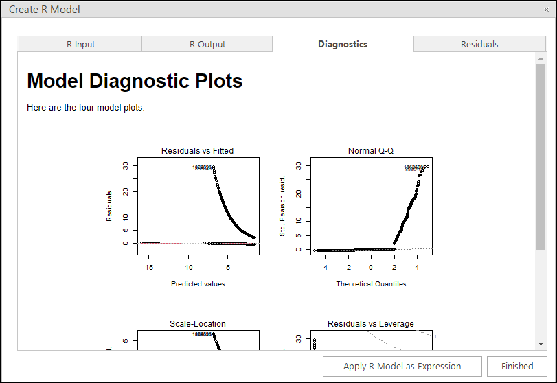

Notes

FastStats provides two environment variables that you can use in your R Markdown file:
- @DATAFRAME is the dataframe of FastStats data passed to R.
- @MODEL is the model object itself.
The file name will be used as the label on the tab when displaying results in the R Model interface.
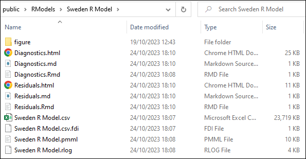
A report will be created for each Rmd file in the RModels folder.
An HTML copy of the report will also be placed in the sub-folder for that model within the RModels folder.

Example reports¶

Model diagnostics¶

This shows four charts plotting different characteristics of the model.

Markdown

---
title: "R Model Plots"
author: "{your name}"
date: "{insert date here}"
output: html_document
---

```{r setup, include=FALSE}
knitr::opts_chunk$set(echo=TRUE)
```
# Model Diagnostic Plots

Here are the four model plots:

```{r plots, echo=FALSE}
par(mfrow = c(2,2))
plot(@MODEL)
```

Model residuals¶

This shows a chart of the residuals for each input variable in the model.

Markdown

---
title: "R Model Plots"
author: "{your name}"
date: "{insert date here}"
output: html_document
---

```{r setup, include=FALSE}
knitr::opts_chunk$set(echo=TRUE)
```
## Model residuals

Residuals:

```{r plots, echo=FALSE}
par(mfrow = c(2,2))
whichVars <- names(@DATAFRAME)
whichVars <- whichVars[c(-1)]
for (V in whichVars) {
  plot(@DATAFRAME[[V]], resid(@MODEL), main = V, xlab = "", pch = 16)
}
```

Note

This StackOverflow answer is a very helpful explanation to understand R Markdown and how the rmarkdown package renders these reports.