Scenarios

In all cases (including standard modelling), the Modelling Environment identifies the differences between two groups of customers - the Analysis and Base - and uses these differences to build a model that predicts who is most likely to be in the Analysis selection.

For example, in a simple campaign response scenario, the Analysis selection might be people who both received the campaign and responded; they could be compared against a Base selection of people who just received the campaign.

In an alternative scenario with 3 events - "communication-booking-cancellation" - the Analysis selection of people who have experienced the complete sequence could be compared against a Base selection of:

• people who just received the communication or
• people who received the communication, booked a holiday (but didn't cancel)

The latter would focus on what is different about people who ultimately cancel.

Essentially the definition of the modelling Analysis/Base scenario involves drawing a line part way through the sequence, such that the model will identify what is different about people who complete the sequence rather than stop short of the line.

Modelling point-in-time¶

Once you have identified the Analysis and Base customer selections, you then need to specify the modelling "point-in-time". It is the behaviour up to this time point that is analysed when determining the differences between the Analysis and Base selections. The choice of this time point depends on what marketing intervention is planned and, therefore, what customer behaviour is available on which to make your marketing decisions.

There are two main types of scenario:

• Firstly, where customers are responding to some existing marketing communication.
• Secondly, where customers are making some spontaneous action, which a possible marketing communication could be designed to encourage/discourage.

Let's consider each type of scenario in turn.

Scenario 1: Campaign response¶

In the first type of scenario, there is an existing marketing communication, and the purpose of modelling is to gain insight from customer behaviour up to the date of the campaign in order to improve your decision of who to include in the campaign next time.

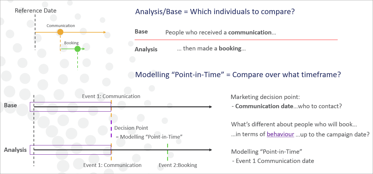
The model might, for example, identify that people who have recently made a booking are unlikely to respond since they already have a holiday booked. In this case the modelling time point would be Event 1.

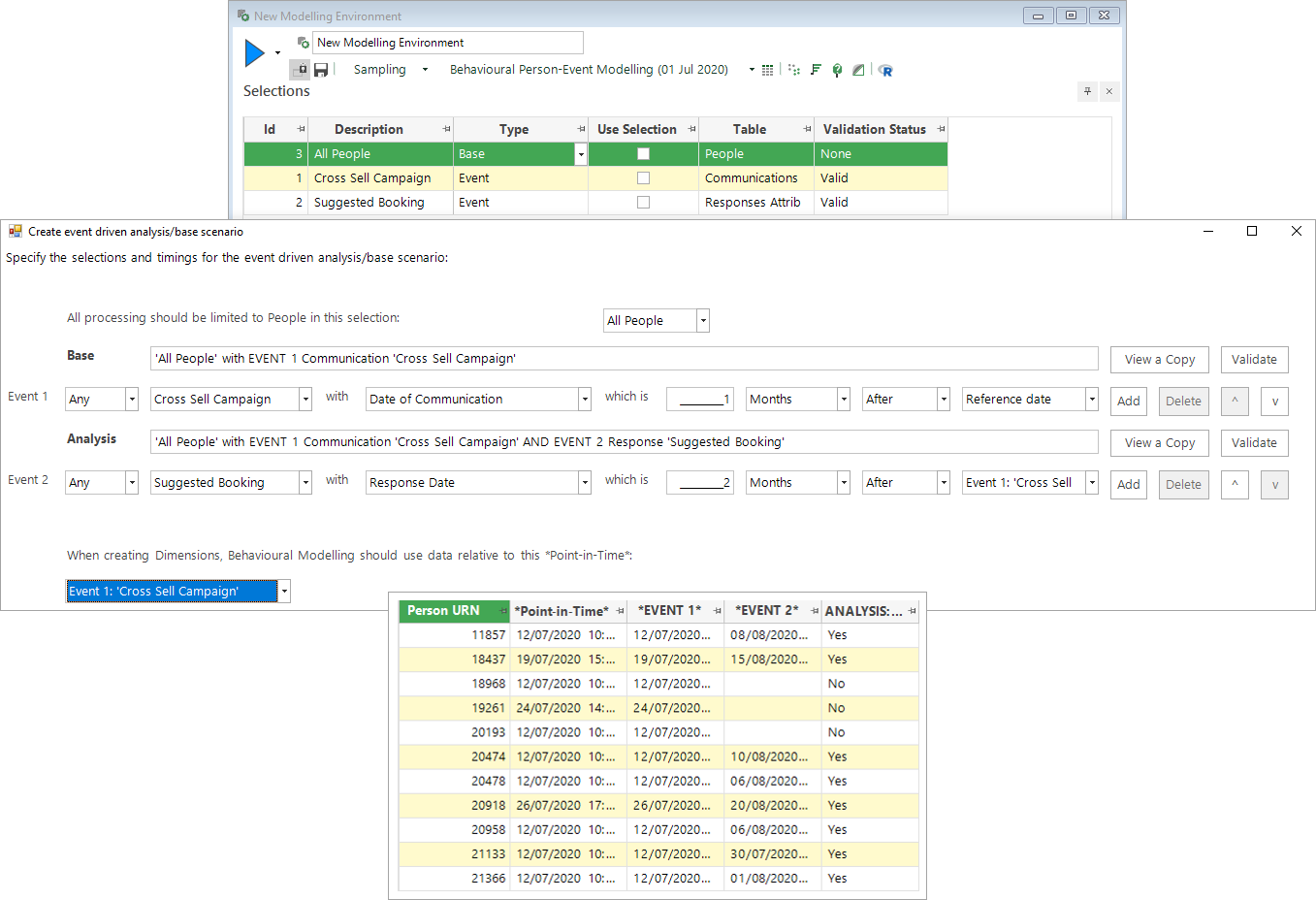
The data grid confirms that the point in time used for modelling corresponds with the time of Event 1 for people in both the Analysis and Base groups.

Scenario 2: Spontaneous action¶

In the second type of scenario, there is no existing communication but, instead, there is the possibility of sending a communication to people who look like they might cancel. The sequence here might be - make a booking...take out insurance...cancel.

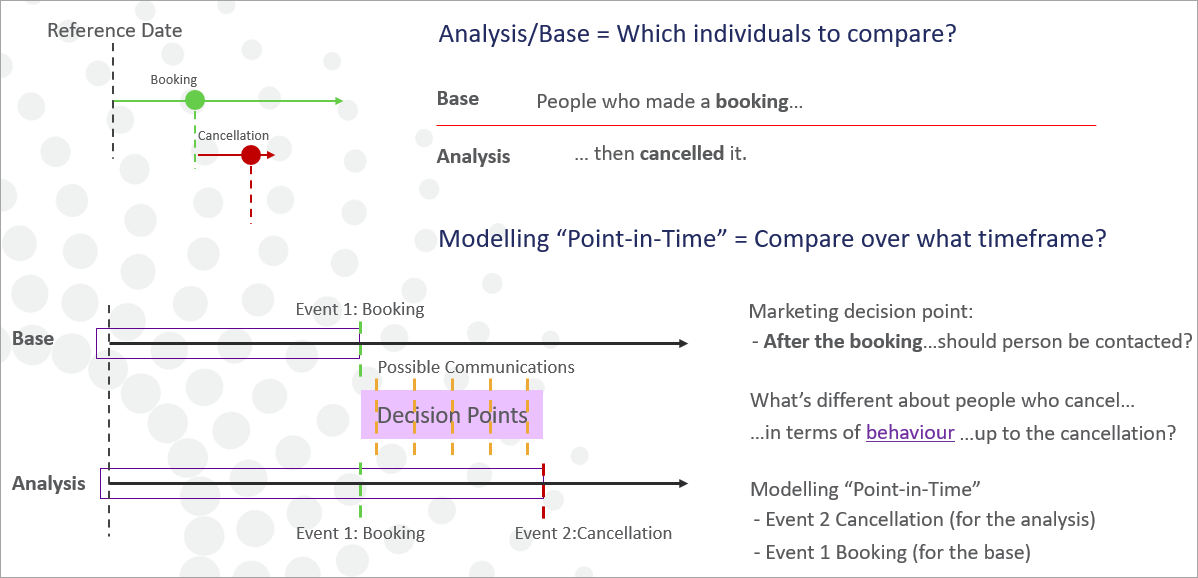
Here you need to understand the behaviour right up until the date people cancel. For example, a model might identify that the people who cancel have been very active in the days leading up to cancellation - perhaps checking out reviews on the website, or contacting a call centre.

In this case, your modelling time point needs to be set at Event 2 - i.e. the cancellation date - to examine behaviour immediately before cancellation. This creates a need for additional information about people in your Base selection, to specify the behaviour to examine since, by definition, they do not have a cancellation date. In the user interface, you should pick one of the earlier events (such as the Booking Date).

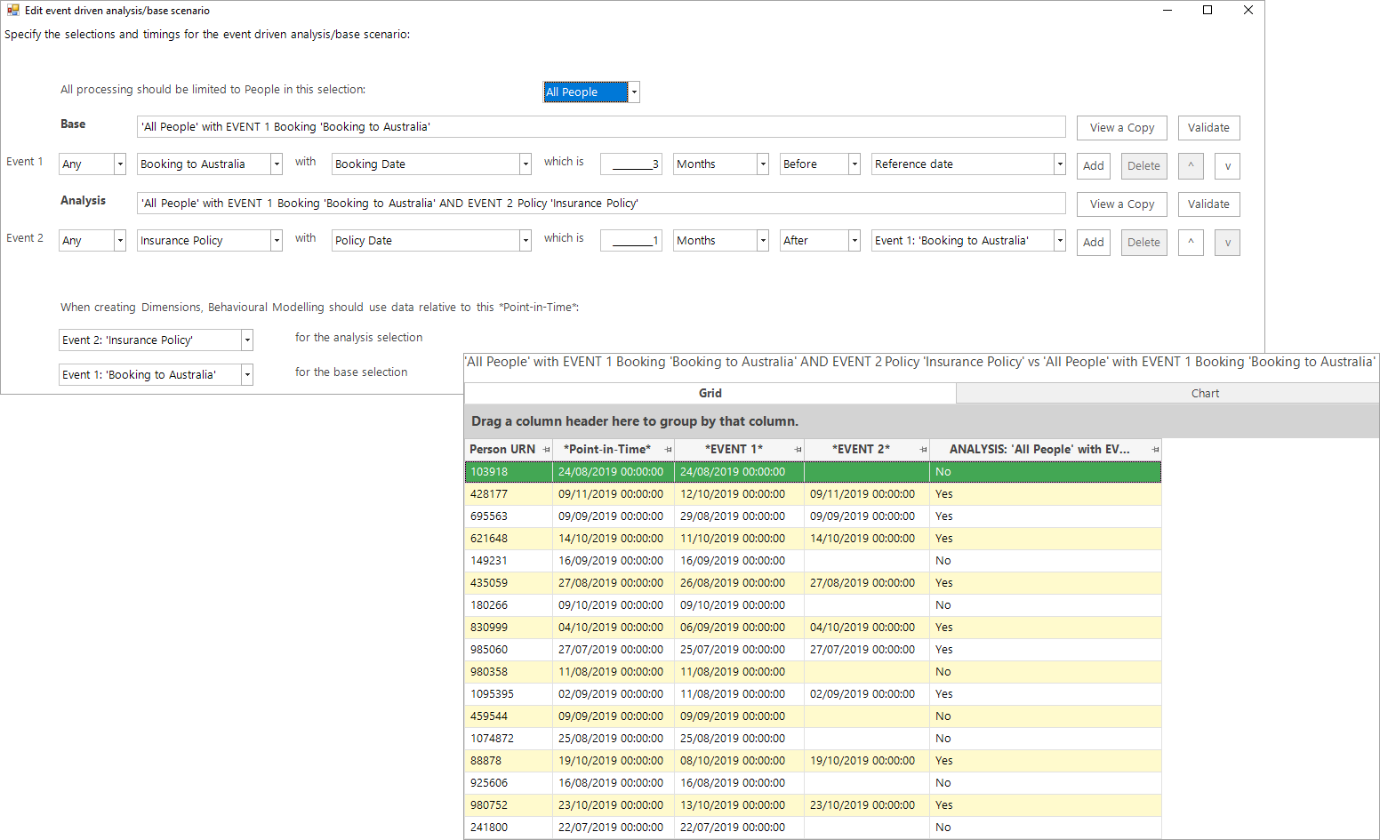
The data grid below shows that the point in time is:

• Policy Date from Event 2 - for people in the Analysis group

• Booking Date from Event 1 - for people with no insurance policy.

  

Extended behavioural modelling selection scenarios¶

Behavioural modelling identifies groups of people who have historically exhibited a specific behaviour - for example, responding to a campaign. You can then analyse how a group's earlier behaviour differs from others, with the aim of predicting which additional people within your database are likely to behave similarly.

Previously, the behaviour being modelled had to involve an active event, such as a response. You can now also model inactive events - the absence of an action - and optionally follow this with any number of subsequent events.

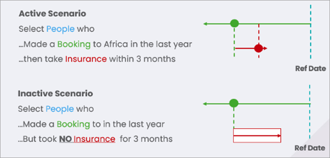
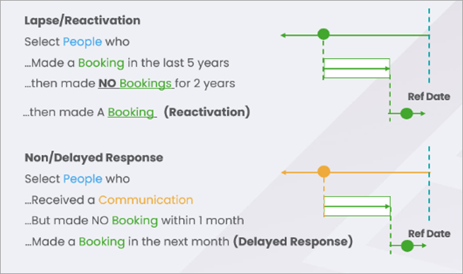
This enables new modelling scenarios to be modelled and allows FastStats to identify people who are likely to exhibit these behaviours, including:

• Lapsing - e.g. People who make a donation but then do not make a donation for 2 years.
• Reactivation - e.g. People who have lapsed but then make another donation.
• Non-responses - e.g. People who receive a communication and do not make a purchase.

• Delayed responses - e.g. People who initially have not responded but then make a response.

  

Further scenarios¶

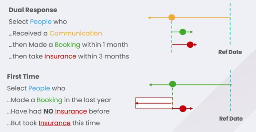
Event sequences are no longer limited to a single linear chain. You can now:

• Allow multiple events to follow the same event.
• Define events as occurring before another event.

This enables scenarios such as:

• Multiple response - e.g. A communication followed by both a booking and the purchase of an insurance policy.

• First-time response - e.g. A communication followed by a purchase of a product that the person had not bought before, or a supporter making a 'regular' donation for the first time after only making ad-hoc donations previously.

  

Set-up¶

Inactive scenarios are set up in the same way as active ones, but use the option "No" to indicate an inactive event.

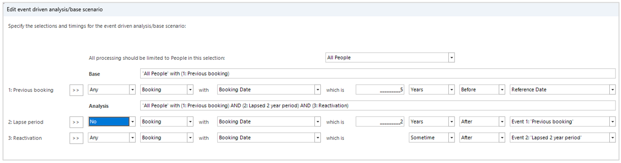
The inactive period must be at least as long as the time specified, but could be longer. The "point-in-time" associated with this event is the "last date checked and free of transactions" (for example, 2 years after event 1). When another event is set as following the inactive period, it can be any time after this "check date".

Implementation and limitations¶

Inactive events¶

Active events use exact calendar units - for example, 1 month after 1^st February = 1^st March.

Inactive events approximate all units into days - for example, no response within a month from 1^st February checks 30 days, reaching up to 3^rd March.

The approximations used always convert units to a whole number of days, rounding down where necessary. So:

1 month = 30 days (30.4)

2 months = 60 days (60.8)

3 months = 91 days

As a result - and as expected - 12 months = 365 days. Leap years are handled so that 3 years = 1095 days, but 4 years = 1461 days.

Inactive events must have a fixed time period - for example, no donation for 2 years. You cannot use the open-ended, "sometime after" option.

Many-to-one events¶

The algorithm used currently may only find a subset of the people who match the given event sequence. Everyone selected will match the sequence, but other people with the sequence may not be selected.

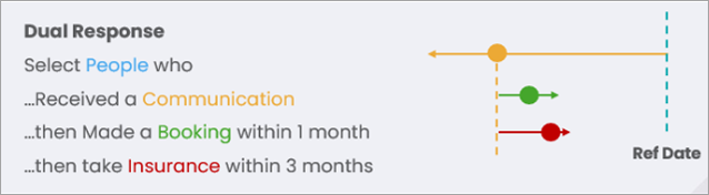
For example, the algorithm will find a pair of transactions where the conditions for Event 1 and Event 2 are satisfied. It then checks to see if Event 3 is also satisfied, but it's possible that Event 3 could still be satisfied if a different pair was chosen. For modelling purposes this is usually fine, as the overall modelling process is to compare an Analysis group of people who meet the conditions of the event sequence against a Base group, and this doesn't need to be everyone who meets the conditions.

To maximise the size of the subset selected, make Event 2 the more restrictive condition relative to Event 3. This means that, once an Event 1-2 pair has been found, it is more likely also to pass the conditions for Event 3.

Maximum 5 years analysed¶

When determining if someone matches an event sequence, you can analyse a maximum of five years' worth of data for each person for each event. The time interval you set in the dialogue informs how much data is needed. For example, to select people who made a donation in the last five years, after two years of inactivity, you actually need to check seven years of data to evaluate the second event. In such cases, a warning is issued in the log. When the data is truncated to 5 years, a person may still be selected if they exhibit the events within that time.

The warning is:

6875 individual level records have some event level data that has been truncated. Each event can only process data spanning up to 1920 days (5.25 years) per individual. Only the earlier events will be analysed when considering an individual for selection.

This is not necessarily a problem as it will depend on the definition of the event whether the truncated data is sufficient to make the selection.

To avoid this warning, limit the possible events per individual by either reducing the interval between events or by adding criteria to restrict the event selection.

Custom event names¶

By default, events are called Event 1, Event 2, etc. but you can now customise the names and descriptions using the >> button. The description updates automatically from the name unless you edit it manually.

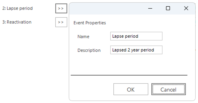
To return to the default description, simply delete the custom description.

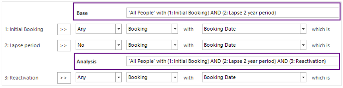
Unless you have manually changed them, the Analysis and Base selection names update automatically when the event names change. To return to the automatic defaults, simply delete the entire manual description.

The position of the boundary between Base and Analysis determines what behaviour is being analysed. In the screenshot above, the model is trying to identify differences in behaviour between people who reactivate and those who simply lapse. You can move events up and down the sequence using the arrow buttons.

Auto-generated selections¶

The sequence of events defined in the selection scenario dialogue are converted into a pair of "Selections" which are then used to define the profiles used in the model. You can see these selections via the "View a Copy" option:

Alternatively, right click on the Selection tab from within the Modelling Environment:

This launches a selection that identifies people matching the event sequence:

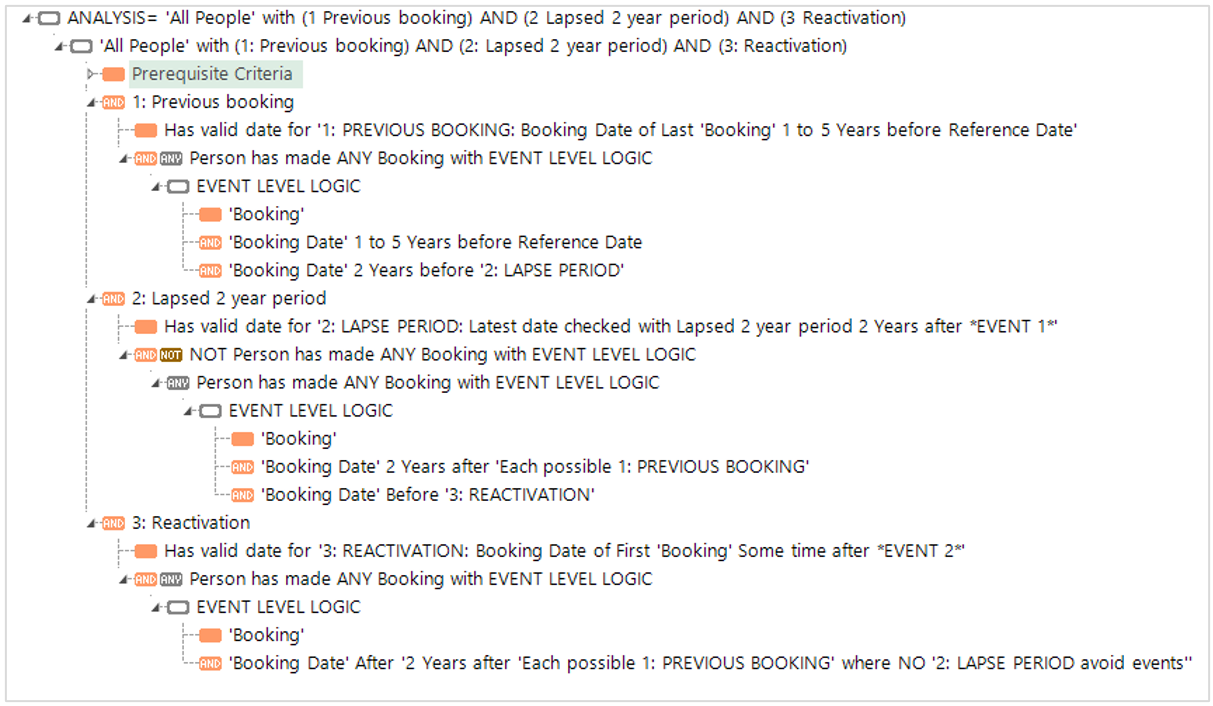
The selection tree combines complex expressions that make the selection with dummy expressions that help to make the overall logic clear.

The top-level nodes contain the logic necessary to select the correct people - those who exhibit the defined sequence of events:

The remaining nodes serve only as labels to indicate how the events are defined. If you click on one of these, it is simply a dummy expression which always returns a 1 or 0, and serves to describe how the event sequence has been defined.

Data grid options¶

You can use a data grid to show the detail behind your selections.

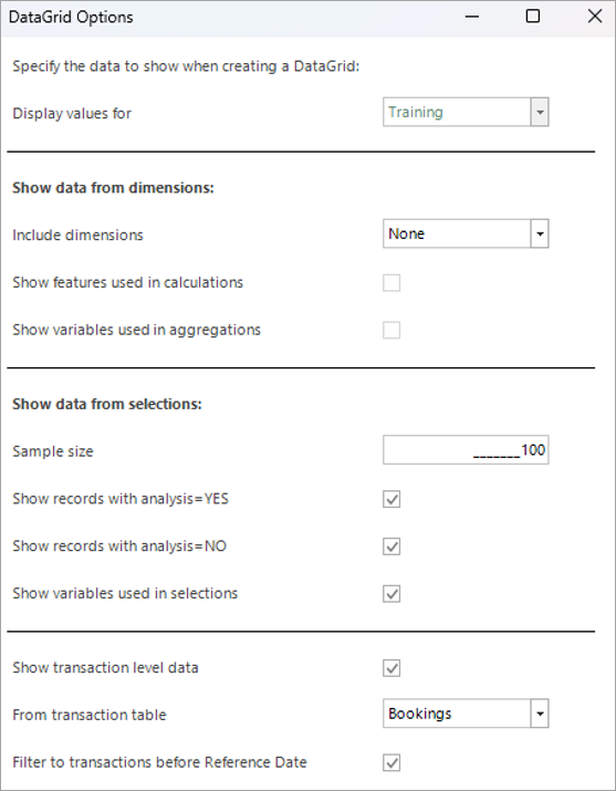
The options for displaying data relating to the dimensions allow:

• Features which are calculations of other features to display these too.
• Transaction level variables used in any aggregation feature.

You can also:

• Specify how many records the Analysis or Non-Analysis to display.
• Automatically extract and display any variable used in the event criteria.
• Set the level of the data grid to one of the transaction tables (or leave at the Person level).
• Add a transaction filter to limit records to before the reference date.

Data is displayed for each of the points-in-time associated with each event, using the custom event name, if specified, along with any transactional variables.

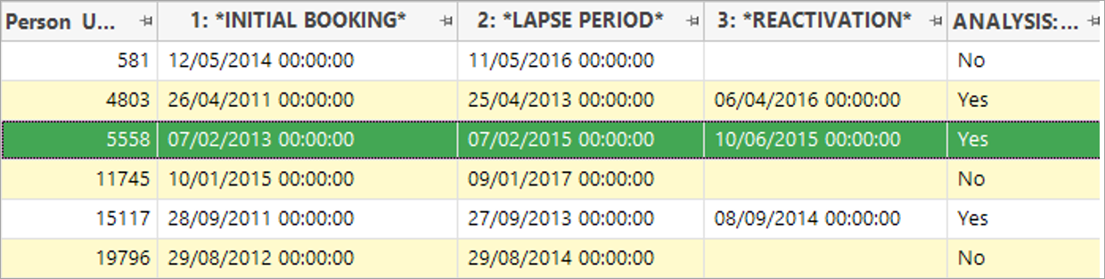
In the above example, all people have had a 2-year lapse period. Note that the date for the second event is the "last date checked and free of transactions" and is, therefore, two years after the initial booking. People in the Analysis selection have the additional reactivation event which corresponds to a subsequent booking.

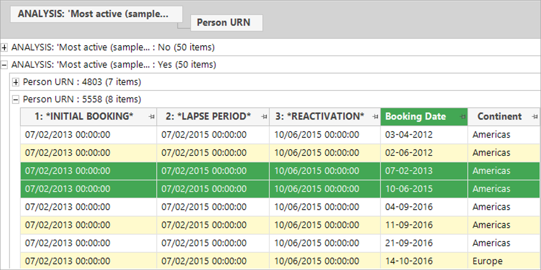
By changing the level of the data grid to bookings, it is possible to see the reason why people have been selected.

This individual had:

An initial booking on 7^th February 2013, followed by at least a 2-year lapse period with no bookings, followed by a reactivation booking on 10^th June 2015.